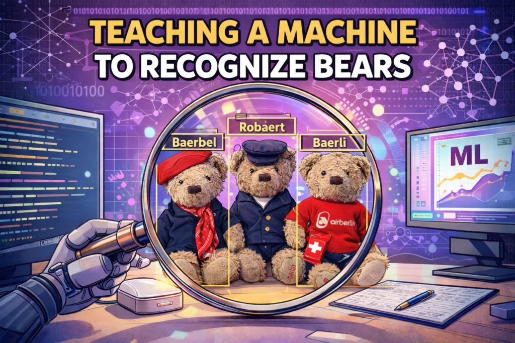
This project did not start as an attempt to build a generic image recognition system or to benchmark computer vision frameworks. It started with three teddy bears that have been traveling with me since 2017.

Over the years, they have accompanied me on flights, through airports, into hotel rooms, conference venues, cafés, and occasionally onto beaches. Airline by airline, the family slowly grew. Each bear developed its own character, its own role, and eventually its own name. They are not famous on Social Media, and they were never meant to be. They exist mainly in my camera roll and in the small stories I write about them after a trip for their Instagram (https://www.instagram.com/flywiththebears/)

Writing those stories has always been a manual and very personal process. I scroll through photos, remember where we were, notice what the bears were doing, and translate that into short narratives. At some point, I started wondering whether I could support this creative process with a bit of technical assistance. Not to automate the writing itself, but to reduce the friction at the start. Simple notes such as which bear appears in an image, whether there are multiple bears present, or what kind of situation the photo captures would already help me get into the right mindset more quickly.

That question led to a deceptively simple idea. Could a machine help me recognize my bears in travel photos so that I could focus more on the storytelling and less on sorting and scanning images?

At first glance, this looks like a straightforward image classification problem. There are only a few bears, each with a distinct name. The input is an image, the output is a label like Baerli, Baerbel, or Robaert. In practice, it turned out to be a compact but very instructive example of how real-world machine learning systems are designed, evaluated, and iterated on.

The images were not clean product shots. They were travel photos with cluttered backgrounds, inconsistent lighting, varying camera angles, and sometimes more than one bear in the frame. In other cases, there was no bear at all. These details mattered, because they quickly exposed the gap between a toy machine learning example and a system that actually works on real data.

What follows is a description of what was built, what was tested, and what was learned along the way, using a very small and very personal problem as a lens to explore how applied machine learning works in practice

---

From Idea to Problem Definition

The first version of the problem was deliberately simple. I started with a classic directory layout containing training, validation, and test images. Each directory had subfolders named after the bears. From a machine learning point of view, this is the textbook entry point into supervised image classification. An image placed in the Baerli folder represents the class Baerli. An image in the Robaert folder represents Robaert. Most modern frameworks are built to work exactly like this, and for good reason. It removes ambiguity and allows you to focus on model behavior rather than data plumbing.

That formulation works well as long as the data behaves the way the abstraction assumes. Mine did not.

These were not curated product shots or carefully staged portraits. They were travel photos taken in passing. In some images the bear was clearly visible and filled most of the frame. In others it was sitting somewhere in the background, partially hidden behind a coffee cup or a seat armrest. Sometimes two bears appeared together. In a few cases there was no bear at all, just the environment they usually travel through.

This difference is not cosmetic. It goes straight to the core of how classification models work. A classifier trained on labeled images has no notion of absence. It is designed to always choose one of the known classes. If you show it a photo of a beach with no bear in sight, it still has to decide whether that image looks more like Baerli or Baerbel or Robaert. When it does so with high confidence, that is not a failure of the model. It is the expected outcome of the problem formulation.

Realizing this early turned out to be important. It made it clear that the issue was not model quality or parameter tuning, but the structure of the problem itself. The system needed a way to reason about whether a bear is present at all and how many, before it could reasonably decide which bear it was looking at. That insight directly influenced the architecture that followed and ultimately led to separating detection from identification instead of trying to force everything into a single classification step.

---

Establishing a Reproducible Training Setup

Before addressing those conceptual issues, the first priority was to establish a training setup that was both reproducible and observable. The objective was not simply to produce a working model, but to understand how different design choices affected the outcome. That meant being able to compare models, vary parameter settings in a controlled way, and evaluate not only accuracy but also operational characteristics such as inference latency.

To support this, MLflow was used as the experiment tracking backbone. Each training run logged the relevant configuration parameters, training loss curves, validation accuracy, test accuracy, and latency measurements. In addition, all relevant artifacts were stored alongside the metrics, including trained weights, exported ONNX models, and the class index mappings. This turned model training into something that could be inspected, compared, and revisited later, rather than a sequence of isolated experiments that only made sense while they were running.

With that foundation in place, three different model architectures were evaluated as initial candidates. A ResNet50 served as a well-understood convolutional baseline. EfficientNet-B0 was chosen as a modern, parameter-efficient alternative. A Vision Transformer with a base configuration was included to test whether a more recent architecture would offer advantages even on a relatively small dataset. All three models were trained on the same data splits with comparable augmentation strategies to ensure that differences in results could be attributed to the models themselves rather than to experimental noise.

The results were informative in a very practical way. The Vision Transformer performed poorly on both validation and test data. Given the limited size and variability of the dataset, this was not particularly surprising. Transformer-based models tend to benefit from large amounts of data and can struggle to generalize when that condition is not met. ResNet50 produced stable and reasonably accurate results and had low inference latency, which made it a solid baseline. EfficientNet-B0, however, stood out. It consistently achieved higher accuracy on validation and test data while remaining fast enough to be used without hesitation in downstream applications.

That combination of accuracy and performance removed any real ambiguity. EfficientNet-B0 was selected as the identity classifier to move forward with, registered in the experiment tracking system, and exported as an ONNX model for use outside the training environment.

---

Exportability as a First-Class Requirement

From the beginning, one requirement was non-negotiable. The trained model could not remain tied to the environment in which it was created. It needed to be portable and runnable elsewhere, including outside Python and inside systems such as Java applications.

To support this, ONNX was chosen as the interchange format. After training, the EfficientNet model was exported to ONNX together with a small JSON file that preserved the mapping between class indices and bear names. This pairing turned out to be both simple and robust. The ONNX model could be loaded with ONNX Runtime in Python or Java, and the preprocessing steps could be reproduced in a deterministic way without relying on the original training code.

A small inference script was enough to verify that the approach worked. When given a clear image containing a single bear, the exported model produced the correct identity with high confidence. At that point, both the training setup and the export pipeline had proven that they behaved as intended.

---

Confronting Reality: When Classification Is Not Enough

The next step was to move beyond controlled test cases and run the system on more realistic images. That is where the limitations became immediately visible.

The first issue appeared in images containing more than one bear. When two bears were present in the same photo, the classifier tended to focus on one of them and ignore the other. In some cases the prediction shifted depending on background elements rather than the bears themselves. This behavior was not surprising, since the model had only ever been trained to assign a single label to an entire image and had no concept of multiple instances.

The second issue was more fundamental. When an image contained no bear at all, the classifier still produced a confident prediction. Sometimes it was confidently wrong. This again was not a defect in the implementation or the training process. It was the direct consequence of how classification models work. Given a fixed set of classes, the model is forced to choose one, even when none of them truly apply.

At that point it became clear that adjusting confidence thresholds or adding heuristics would only mask the symptoms. The real problem was structural. The system lacked any mechanism to determine whether a bear was present in the image in the first place, and where it was located if it was.

---

Separating Detection from Identification

This insight led to a clear architectural separation. Rather than trying to force a single model to handle every aspect of the problem, the system was split into two distinct stages, each with a well-defined responsibility.

The first stage performs object detection. Its purpose is to determine whether a bear is present in the image at all and, if so, how many bears appear and where they are located. The second stage performs classification. It operates on cropped images of individual bears and decides which specific bear is being shown.

This separation resolves several issues at once. If the detector finds no bears, the correct outcome is simply that no bear is present. If it detects more than two bears, a straightforward business rule can return the label Crew without invoking any classification logic. When one or two bears are detected, each cropped region can be passed independently to the identity classifier, producing stable and interpretable results.

This structure closely reflects how many production-grade vision systems are designed. Detection establishes presence and location. Classification determines identity. Separating these concerns simplifies reasoning about system behavior and makes each component easier to train, evaluate, and evolve independently.

---

Choosing the Detection Stack and Handling Practical Constraints

When it came to detection, licensing and environment stability became first-class concerns. Some widely used detectors are distributed under licenses that complicate reuse in downstream systems, especially when models are exported, embedded, or deployed as part of a larger application. Others rely on dependency stacks that are fragile on Windows, particularly when combined with strict NumPy version constraints.

To avoid both legal and operational friction later on, an Apache-licensed detector was selected. YOLOX turned out to be a good fit. It offers a modern detection architecture, supports export to ONNX, and keeps its dependency footprint within reasonable bounds. This made it suitable not only for experimentation, but also for reuse beyond the initial training environment.

Getting the detector up and running also reinforced another practical lesson. Tooling issues matter. Dependency conflicts, NumPy pinning, Windows path length limitations, and crashes in annotation tools all surfaced during setup. None of these problems are especially interesting on their own, but they are part of the reality of applied machine learning. Ignoring them does not make them disappear, and solving them is a prerequisite for building systems that actually run.

For annotation, a browser-based and containerized approach was chosen to avoid local GUI and library conflicts altogether. Running CVAT in Docker provided a stable and predictable environment for labeling bounding boxes across training, validation, and test images, without entangling the rest of the toolchain in additional dependencies.

---

Training and Evaluating the Detector

With annotated data in place, the detector was trained to recognize a single class, bear. The evaluation did not focus on achieving perfect bounding box alignment, but on whether the detector reliably identified bears across a wide range of scenes and conditions. Robustness mattered more than pixel-level precision, since the downstream classifier only required a reasonable crop to operate correctly.

After training, the detector was exported to ONNX as well. At that point, both stages of the pipeline were portable and independently versioned. The detector’s responsibility is to produce bounding boxes. The classifier’s responsibility is to assign identities. The logic that connects the two is deliberately simple and deterministic, which makes the overall system easier to reason about, test, and extend.

---

What This Project Demonstrated

Several broader lessons emerged from this exercise.

First, model choice only makes sense in context. EfficientNet-B0 was not inherently superior to the other architectures that were tested. It was simply the best fit for this particular dataset size, this specific task, and the performance characteristics that mattered in practice.

Second, individual metrics are rarely sufficient on their own. Validation accuracy in isolation provided an incomplete picture. Only by looking at validation accuracy, test accuracy, and inference latency together did the trade-offs become clear and defensible from an engineering perspective.

Third, architectural decisions outweigh clever tuning. No amount of threshold adjustment or post-processing could compensate for the absence of a detection stage. Once detection was introduced, several of the previously observed failure modes disappeared as a direct consequence of the system design rather than improved model behavior.

Fourth, reproducibility and exportability are not secondary concerns. Treating experiment tracking, model registration, and artifact export as first-class requirements from the beginning transformed what could have remained a one-off experiment into a system that can be reused, extended, and reasoned about over time.

---

Why This Was Worth Doing

At the surface level, this project helps identify which bear appears in which travel photo. Even that small capability already reduces friction when organizing images and starting to write their stories. At a deeper level, it became a compact and surprisingly effective laboratory for understanding how real machine learning systems are built.

The work spanned the full lifecycle, from problem formulation and data preparation to model comparison and deployment considerations. Along the way, theoretical expectations met practical failure modes, and simple assumptions were repeatedly challenged by real data. The exercise reinforced a familiar but often forgotten lesson. Applied machine learning is less about individual algorithms and more about systems, constraints, and iteration.

In the end, it also served as a reminder that some of the most valuable learning projects start with a slightly absurd personal question. If that question is pursued seriously, it can lead to a very concrete understanding of how things actually work.

If nothing else, my bears now travel not only with me, but through a small and well-instrumented machine learning pipeline that knows who they are and when they are present. That feels like a good outcome.